Landslide Risk Assessment from Failure to Consequence
A subset-simulation and large-deformation framework propagates uncertain soil-strength parameters through slope failure and post-failure response, then links case-specific consequence measures to vulnerability, temporal exposure, and risk.
Quantitative risk · Large deformation · Rare-event simulation
This study replaces the usual break between slope-stability analysis and empirical runout estimation with a Coupled Eulerian–Lagrangian (CEL) simulation of pre-failure behavior and post-failure motion. In the runout-to-structure formulation, subset simulation estimates the probability that a realization reaches the specified element, while CEL-derived response quantities enter a separate vulnerability model. In the Ganjingzi application, the consequence measure is instead simulated wave height, with zero vulnerability assigned to stable or blue-alert states. (Cui et al., 2022)
From failure to risk: conceptual boundaries
The paper is not a regional susceptibility-mapping study. It evaluates the risk posed by a specified slope to a specified exposed element. Its central distinction is between a slope that becomes unstable and a realization whose motion reaches the element at risk. (Cui et al., 2022)
| Concept | Meaning in this study | Representation |
|---|---|---|
| Susceptibility | Spatial tendency toward landsliding; not a direct output of this paper | Outside the case-specific QRA |
| Failure | A sampled slope realization becomes unstable | $P_f=N_f/N_t$ |
| Reach probability | A failed landslide reaches the exposed element | $P_r=N_r/N_f$ |
| Impact probability in the runout-to-element formulation | A sampled realization fails and reaches the element; the Ganjingzi wave application uses the separate accounting convention reported in Table 7 | $P_{fr}=N_r/N_t=P_fP_r$ |
| Intensity | Attributes used to characterize the action on the exposed element | CEL-derived velocity, moving volume, and debris depth with prescribed slope height; wave height in the reservoir case |
| Vulnerability | Conditional degree of loss under the modeled intensity and resistance | $V\in[0,1]$ |
| Temporal exposure | Probability that the element is present in the potential impact zone | $P_t$ |
| Risk | Impact probability combined with exposure and conditional loss | $R=P_{fr}P_t\overline{V}E$ |
Here, “impact” primarily means satisfying the reach condition defined for the exposed element. CEL does not directly compute structural damage. It computes motion and intensity measures, which are subsequently converted to vulnerability through empirical functions, engineering judgment, historical information, or assigned wave-alert categories. (Cui et al., 2022)
From slope failure to impact probability
The conventional case-specific risk expression separates slope failure from spatial reach:
Because $P_fP_r=N_r/N_t$, the paper defines a joint failure-and-reach probability:
\[P_{fr}=\frac{N_r}{N_t}, \qquad R=P_{fr}P_t\overline{V}E, \qquad \overline{V}=\frac{1}{N_r}\sum_{j=1}^{N_r}V_j.\]Interpretation. $N_t$ is the total number of sampled slopes, $N_f$ is the number that fail, and $N_r$ is the number that reach the exposed element. The proposed formulation embeds failure and spatial reach in $P_{fr}$; it does not remove failure mechanics from the simulation. Eqs. (2), (9)–(11) from (Cui et al., 2022).
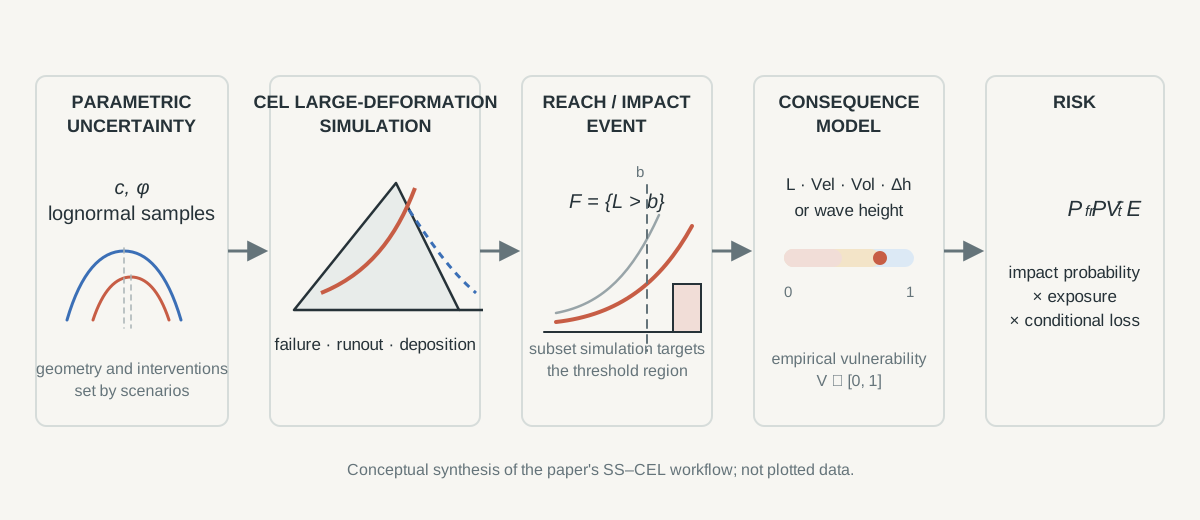
The impact event used by subset simulation
Subset simulation defines the target threshold event as
where $\mathbf{X}$ contains the uncertain soil parameters, $L$ is the CEL-simulated runout distance, and $b$ is the distance from the original slope toe to the exposed element. The paper’s “failure event” in the subset-simulation equations is therefore a mathematical threshold-exceedance event, not merely the initiation of geotechnical failure.
Intermediate events progressively approach the target:
\[F_i=\{z(\mathbf{X})>b_i\}, \qquad b_1<b_2<\cdots<b_n=b,\]with $P(F_1)=P(F_{i+1}\mid F_i)=P_0$. Samples that satisfy the current intermediate event seed Markov-chain Monte Carlo sampling at the next level. Eqs. (12)–(13) from (Cui et al., 2022).
The formal construction partitions the response space into mutually exclusive regions. $\Omega_0$ lies below the first intermediate threshold, $\Omega_i=F_i\setminus F_{i+1}$ for $i=1,\ldots,n-1$, and $\Omega_n=F_n$. Their reported occurrence probabilities are $P(\Omega_i)=P_0^i-P_0^{i+1}$ for $i=0,\ldots,n-1$ and $P(\Omega_n)=P_0^n$. These regions are then weighted by their occurrence probabilities, within-subset proportions of impacting samples, and mean vulnerabilities. (Cui et al., 2022)
This is a probability-weighted aggregation across subset regions, not a simple average of all numerical simulations. Eq. (16) from (Cui et al., 2022).
CEL as the large-deformation engine
CEL combines two numerical descriptions. In the Lagrangian step, the mesh and material deform together. In the Eulerian step, the convective motion is calculated and material and field variables are mapped back to a regular mesh. This two-step treatment avoids the severe mesh distortion that can stop conventional Lagrangian calculations during very large deformation. (Cui et al., 2022)
The first expression is solved in the Lagrangian step; the second represents the Eulerian convective step. The simulations use a linear-elastic, perfectly plastic Mohr–Coulomb material, zero dilation, and ABAQUS CEL. Eqs. (7)–(8) from (Cui et al., 2022).
CEL is the large-deformation implementation used in these cases, but the risk formulation is not tied to it; the authors note that other large-deformation solvers could be substituted. (Cui et al., 2022)

What is uncertain—and what is prescribed
The case studies propagate parametric uncertainty in cohesion $c$ and friction angle $\phi$, both modeled as lognormal random variables. The paper does not state that they are statistically independent. Unit weight, stiffness, Poisson’s ratio, geometry, excavation angle, reservoir level, and remediation configuration are prescribed inputs or scenarios. Natural spatial variability is not modeled. (Cui et al., 2022)
| Case | Random soil-strength parameters | Representative fixed/scenario inputs |
|---|---|---|
| Baqiao | $c$ and $\phi$ for Lishi and Malan loess | Loess stratigraphy, excavation geometry, structure location, $E$, $\nu$, and unit weight |
| Ganjingzi | $c$ and $\phi$ for the sliding mass | Global/local geometry, 145/175 m water levels, anti-slide piles, interfaces, $E$, $\nu$, and unit weight |
| Case and material | $\gamma$ (kN/m³) | $E$ (MPa) | $\nu$ | $\phi$, mean ± SD | $c$, mean ± SD |
|---|---|---|---|---|---|
| Baqiao — Lishi loess $Q_2$ | 18.0 | 85 | 0.31 | 23.6° ± 3.1° | 42.1 ± 20.5 kPa |
| Baqiao — Malan loess $Q_3$ | 17.1 | 68 | 0.30 | 21.5° ± 4.75° | 30.5 ± 17.7 kPa |
| Ganjingzi — sliding mass | 23.6 | 3.2 | 0.33 | 29.8° ± 3.17° | 18.5 ± 2.1 kPa |
| Ganjingzi — bedrock | 26.2 | 1,600 | 0.49 | Not reported | Not reported |
Three analytical routes in the paper
The efficiency and method-comparison results use three distinct routes. Keeping them separate is essential:
| Route | Composition | Purpose | Consequence information |
|---|---|---|---|
| Proposed Approach 1 | Subset simulation + CEL | Formal QRA method proposed in the paper | Scenario-specific $L$, velocity, volume, debris depth or wave height |
| Direct MCS + CEL | Direct Monte Carlo sampling + the same CEL model | Numerical validation of SS estimates and sampling efficiency | The same CEL-derived dynamic quantities |
| Conventional Approach 2 | 10,000 MCS samples + SRFEM stability + empirical runout | Framework comparison in Baqiao | Runout is estimated empirically; post-failure velocity and deposit evolution are not directly simulated, and $V=1$ is assumed after reach |
Baqiao: excavation, runout, and structural risk
Site and controlled excavation scenarios
The 2011 Baqiao loess landslide was approximately 90 m high and 170 m wide, with a 12 m slip-surface thickness, a sliding volume of $1.5\times10^5$ m³, and an observed runout of 150 m. Two nearby structures were destroyed. Field investigation identified slope-toe excavation for brick-making material as the triggering factor considered in the case study. (Cui et al., 2022)

| Scenario | Slope angle | Structure threshold $b$ | Mean-parameter FS | Role |
|---|---|---|---|---|
| I | 24.3° | — | 1.32 | Original state; not included in the SS risk comparison |
| II | 40° | 40 m | 1.04 | First excavation scenario |
| III | 50° | 66 m | 0.87 | Intermediate excavation |
| IV | 60° | 82 m | 0.75 | Steepest excavation |
The modeled element at risk is a three-floor steel structure no more than five years old. Its resistance score is
\[Res=(0.90\times0.65\times0.80)^{1/3}\approx0.78,\]based on structural type, floor count, and age. In the Baqiao comparison, $P_t=1$ and $E=1$ monetary unit. The resulting $R$ is therefore a comparative risk value under those assumptions, rather than a site-specific estimate of monetary loss. (Cui et al., 2022)
From CEL dynamics to structural vulnerability
The Baqiao vulnerability model first combines moving volume, velocity, debris depth, and slope height into a dimensionless intensity $Int$. It then compares intensity with the resistance score:
Let $x=Int/Res$. Then
\[V= \begin{cases} 2x^2, & x\le0.5,\\[3pt] 1-2(1-x)^2, & 0.5<x\le1,\\[3pt] 1, & x>1, \end{cases}\]with
\[Int=1-\prod_{k=1}^{n}(1-\alpha_k), \qquad Res=\left(\prod_{k=1}^{n}\beta_k\right)^{1/n}.\]$\alpha_k$ are intensity-factor scores and $\beta_k$ are resistance-factor scores assigned from the paper's vulnerability table. Eqs. (17)–(19) from (Cui et al., 2022).
Slope cutting shifts the simulated distributions of runout distance, velocity, and moving volume toward larger values:
| Scenario | Runout distance, mean ± SD | Velocity, mean ± SD | Moving volume, mean ± SD |
|---|---|---|---|
| II | 14.10 ± 16.75 m | 1.07 ± 1.04 m/s | $(0.35\pm0.49)\times10^5$ m³ |
| III | 39.00 ± 23.93 m | 2.43 ± 1.71 m/s | $(1.14\pm0.83)\times10^5$ m³ |
| IV | 58.46 ± 26.52 m | 3.11 ± 1.06 m/s | $(1.95\pm0.93)\times10^5$ m³ |

A worked subset-simulation calculation
For Scenario II, the paper sets $P_0=0.1$ and $N=400$ per level. One initial direct-MCS level and two MCMCS levels require
\[400+(1-0.1)\times2\times400=1{,}120\]simulations. At each of the first two levels, the 40 samples with the largest runout distances become seeds for the next level. (Cui et al., 2022)
| Subset | $P(\Omega_i)$ | Impacting samples | $P_{fr,i}$ | $\overline{V}_i$ |
|---|---|---|---|---|
| $\Omega_0$ | 0.90 | 0/360 | 0 | 0 |
| $\Omega_1$ | 0.09 | 285/360 | 0.792 | 0.955 |
| $\Omega_2$ | 0.01 | 400/400 | 1.000 | 0.981 |
The weighted calculation gives $P_{fr}\approx0.081$ and $R\approx0.078$; Table 4 reports impact probability 8.13%, mean vulnerability 0.958, and risk 0.078. This worked example shows how rare-event probability and conditional consequence are assembled rather than merely reporting a simulation count. (Cui et al., 2022)
Risk, direct-MCS validation, and the empirical comparator
| Scenario | $P_{fr}$ | $\overline V$ | SS–CEL $R$ | Direct MCS–CEL $R$ | Reaching samples / CEL runs (unweighted) |
|---|---|---|---|---|---|
| II | 8.13% | 0.958 | 0.078 | 0.081 | 685/1,120 |
| III | 11.75% | 0.958 | 0.113 | 0.109 | 407/760 |
| IV | 14.75% | 0.964 | 0.142 | 0.143 | 419/760 |
The raw SS count 685/1,120 is not an empirical estimate of $P_{fr}$; samples from different subset levels carry different occurrence-probability weights.
The direct-MCS–CEL values provide numerical validation of subset sampling within the same physical model. For Scenario II, direct MCS required 8,000 CEL simulations to obtain 678 impacting samples, while SS obtained 685 from 1,120. The efficiency comparison is therefore SS versus direct MCS inside the CEL framework—not SS–CEL versus the conventional empirical Approach 2. (Cui et al., 2022)
The conventional comparison produces much larger risk values in this case:
| Scenario | $P_f$ | $P_r$ | Assumed $V$ after reach | Approach 2 $R$ |
|---|---|---|---|---|
| II | 50.70% | 100% | 1 | 0.507 |
| III | 89.30% | 98.43% | 1 | 0.879 |
| IV | 99.75% | 79.18% | 1 | 0.790 |
For Scenario IV, the empirical model predicts mean runout 94.17 m with SD 14.47 m, compared with an 82 m structure threshold. The paper attributes the conservative estimate in this Baqiao comparison to the empirical runout relation, which was derived from a limited set of loess-landslide records spanning different triggering conditions and may therefore be biased and uncertain. Separately, Approach 2 adopts the most unfavorable vulnerability assumption, $V=1$, whenever the modeled runout reaches the structure. This result is specific to the comparator used in Baqiao and is not evidence that every conventional QRA necessarily overestimates risk. (Cui et al., 2022)
Ganjingzi: landslide motion, impulse waves, and passenger risk
Geometry and modeled scenarios
The Ganjingzi slope lies approximately 150 m from the Yangtze River navigation channel. The potential global landslide is about 440 m long, 220 m wide, and 21 m thick, with a volume of $2\times10^6$ m³. The local severe-deformation zone is approximately 170 m by 100 m by 12 m, with a volume of $2\times10^5$ m³. (Cui et al., 2022)

| Scenario | Slope state | Reservoir levels | Consequence pathway |
|---|---|---|---|
| I | Potential global landslide | 145 and 175 m | Water entry → impulse wave → vessel vulnerability |
| II | Potential local landslide | 145 and 175 m | Water entry → impulse wave → vessel vulnerability |
| III | Slope reinforced by two anti-slide-pile rows | 145 and 175 m | Residual wave consequence after remediation |
The CEL model represents bedrock and piles as rigid materials, uses Coulomb-friction soil–pile and soil–bedrock interfaces, applies self-weight, and contains approximately 73,000 EC3D8R elements, for which the paper reports a 2 m $\times$ 2 m element size. Cohesion and friction angle of the sliding mass are lognormal random variables with reported means and SDs of $18.5\pm2.1$ kPa and $29.8^\circ\pm3.17^\circ$. (Cui et al., 2022)
From simulated wave height to vulnerability and exposure
Water-surface trace points convert soil–water motion into maximum wave height. The consequence model then maps wave height to vessel vulnerability: (Cui et al., 2022)
| Wave height | Alert class | Assigned vessel vulnerability |
|---|---|---|
| $>3$ m | Red | 0.8 |
| 2–3 m | Orange | 0.4 |
| 1–2 m | Yellow | 0.2 |
| $\le1$ m | Blue | 0 |
The temporal-exposure calculation uses approximately 200 vessels per day, an assumed vessel speed of 25 km/h, and a 220 m potential impact zone. Each vessel occupies the zone for 31.4 s, giving
This is the probability that passengers are present in the potential impact zone at the moment of a landslide under the paper's traffic assumptions. (Cui et al., 2022)

Reported risk and effect of anti-slide piles
For this case, stable or blue-alert samples are retained and assigned $V=0$. Table 7 therefore lists $P_{fr}=100\%$ for its aggregation. This is an accounting choice for the wave-consequence calculation; it does not mean that every sampled slope produces a damaging landslide. (Cui et al., 2022)
| Scenario | Water level | Reported $P_{fr}$ | $P_t$ | Mean vulnerability | Reported individual risk $R$ | Criterion |
|---|---|---|---|---|---|---|
| Global | 145 m | 100% | 7.27% | 0.022 | $3.12\times10^{-4}$ | Above $10^{-4}$ |
| Global | 175 m | 100% | 7.27% | 0.042 | $6.04\times10^{-4}$ | Above $10^{-4}$ |
| Local | 145 m | 100% | 7.27% | 0.079 | $1.15\times10^{-3}$ | Above $10^{-4}$ |
| Local | 175 m | 100% | 7.27% | 0.112 | $1.62\times10^{-3}$ | Above $10^{-4}$ |
| Reinforced | 145 m | 100% | 7.27% | 0.003 | $3.65\times10^{-5}$ | Below $10^{-4}$ |
| Reinforced | 175 m | 100% | 7.27% | 0 | 0 | Below $10^{-4}$ |
All four unreinforced global/local cases exceed the paper’s adopted individual-risk criterion of $10^{-4}$. The Table 7 values for the reinforced slope are no greater than $3.65\times10^{-5}$. (Cui et al., 2022)
What this work establishes
Evidence-supported contribution
- Failure and runout share one physical simulation. CEL propagates the same sampled shear-strength parameters through initiation, large deformation, travel, and deposition. (Cui et al., 2022)
- For the runout-to-element formulation, the terminal event is impact. In Baqiao, the framework directly estimates $P_{fr}$, the joint probability of slope failure and reach, instead of estimating $P_f$ and $P_r$ separately. In Ganjingzi, all subset states are retained and consequence is controlled through wave-height-dependent vulnerability. (Cui et al., 2022)
- Rare-event sampling is evaluated within a fixed physical model. SS–CEL and direct MCS–CEL produce close Baqiao risk values, while SS generates comparable numbers of impacting realizations with fewer CEL evaluations. (Cui et al., 2022)
- The same chain accommodates different consequences. Baqiao uses structure vulnerability based on runout dynamics; Ganjingzi uses CEL-simulated wave height, vessel exposure, and alert-based vulnerability to compare anti-slide piles. (Cui et al., 2022)
Modeling assumptions stated in the paper
- Soil is linear elastic and perfectly plastic under a Mohr–Coulomb model; dilation is set to zero.
- Cohesion and friction angle are lognormal random variables; case geometry and interventions are prescribed scenarios.
- Field geological conditions are simplified to keep the computational load affordable.
- Baqiao fixes $P_t=1$ and $E=1$ for comparative evaluation.
- Vulnerability is based on empirical functions, engineering judgment, historical records, or assigned wave-alert classes rather than direct simulation of structural impact. (Cui et al., 2022)
Authors’ stated limitations
The paper identifies two principal limitations. First, vulnerability is not obtained from direct landslide–structure impact simulation; such simulation could improve the consequence assessment. Second, natural spatial variability of soil properties is not included, even though prior studies show that it can affect risk. The case studies therefore demonstrate the proposed computational framework under parametric uncertainty and simplified site representations. (Cui et al., 2022)
References
2022
- Acta Geotech.Quantitative risk assessment of landslides with direct simulation of pre-failure to post-failure behaviorsActa Geotechnica, 2022